Polynomials on the Sierpinski Gasket
The space \(\mathcal{H}_j\)
-
Let \(f: SG \mapsto \mathbb{R}\). Then \(f\) is a \(j\)-degree polynomial iff
\(\Delta^{j+1}f = 0\) and \(\Delta^{j}f\neq 0\), i.e \(f\) is \(j\)-harmonic but not \((j-1)\)-harmonic. -
The space of polynomials with degree \(\le j\) is denoted \(\mathcal{H}_{j}\)
-
Let \(f \in \mathcal{H}_j\). Then \(f\) is determined uniquely by the values \((f(q_0), f(q_1), f(q_2), \Delta f(q_0), \Delta f(q_1), \ldots, \Delta^jf(q_2))\)
-
dim(\(\mathcal{H}_j\)) = \(3j + 3\)
-
A natural basis for \(\mathcal{H}_{j}\) is the family of functions \(\{f_{nk}\}\) where \[\Delta^{m}f_{nk}(q_i) = \delta_{mn}\delta_{ki}\]
-
For example, the three harmonic functions \(h_i\) where \(h_i(q_j) = \delta_{ij}\) form a basis for \(\mathcal{H}_0\)
The Monomial Basis
-
We want to mimic the case on \(I = [0,1]\) where we can expand a function as a Taylor series in terms of basis functions where we use derivative information at one point.
-
For example, for harmonic functions, we have the following basis \(\{P_{0k}\}\) where the tuple of values \((u(q_0), \partial_nu(q_0), \partial_Tu(q_0)) = e_k\): \[P_{01} = h_0 + h_1 + h_2 \hspace{0.35in} P_{02} = -\frac{1}{2}(h_1 + h_2) \hspace{0.35in} P_{03} = \frac{1}{2}(h_1 - h_2)\] If \(f \in \mathcal{H}_0\) then \(f = f(q_0)P_{01} + \partial_nf(q_0)P_{02} + \partial_Tf(q_0)P_{03}\)
-
We introduce the following basis \(\{P_{jk}\}\) where \[\begin{aligned} \Delta^nP_{jk}(q_0) &= \delta_{nj}\delta_{k1}\\ \Delta^n\partial_nP_{jk}(q_0) &= \delta_{nj}\delta_{k2}\\ \Delta^n\partial_TP_{jk}(q_0) &= \delta_{nj}\delta_{k3}\\ \end{aligned}\] This is known as the monomial basis.
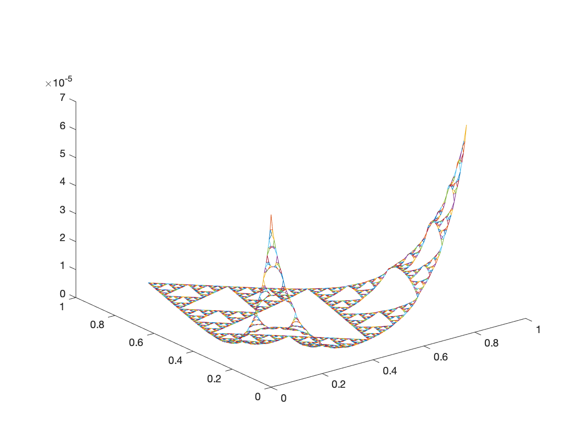
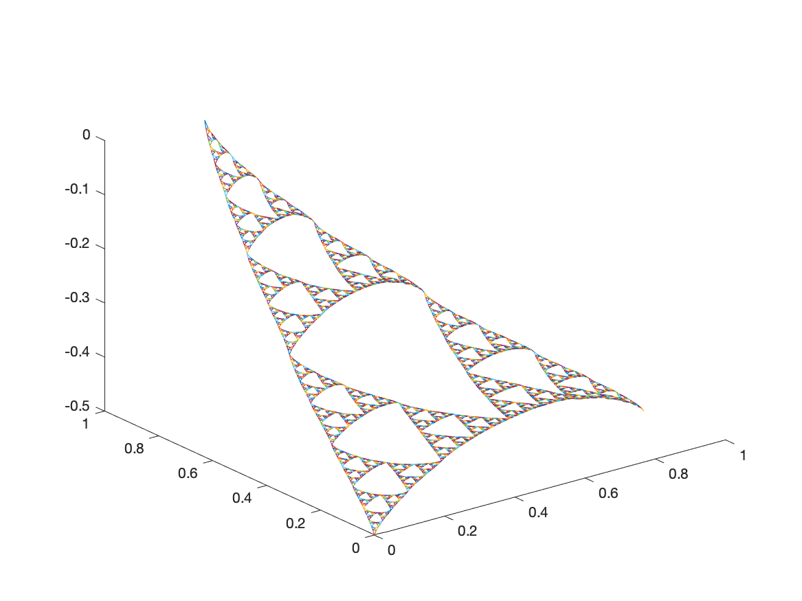
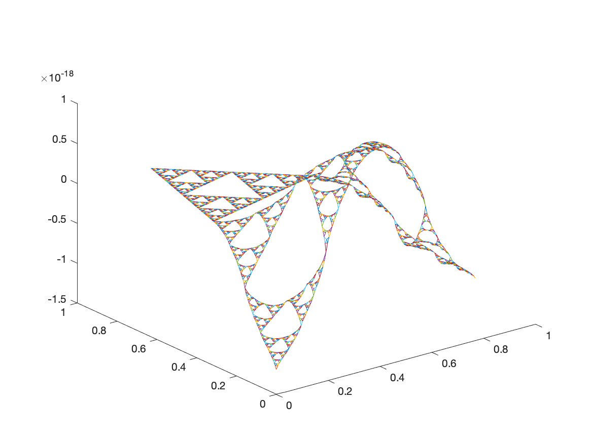
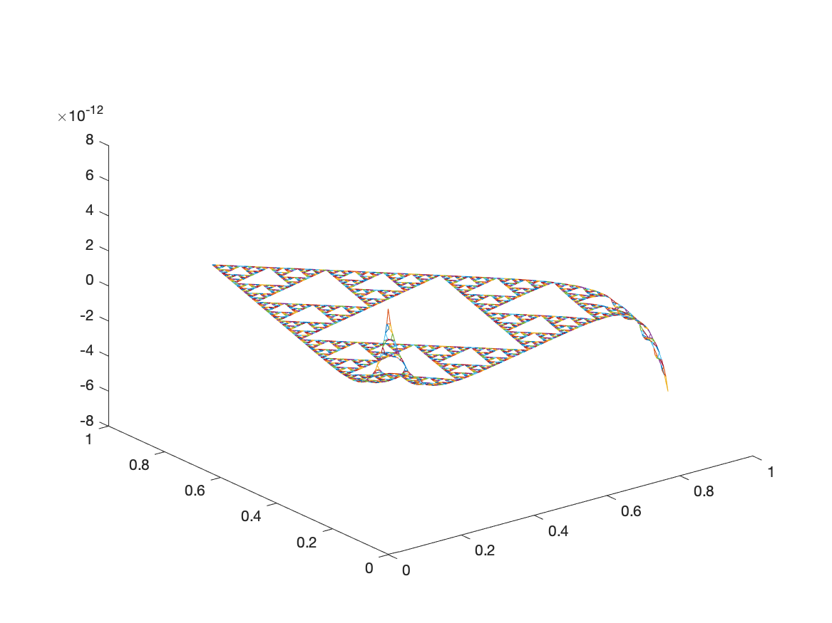
Examples of Monomials
Orthogonal Polynomials
-
The space of polynomials on \(\mathbb{R}\), denoted \(P(\mathbb{R})\) can be endowed with the following inner product: \[\langle f,g \rangle = \int_{\mathbb{R}}f(x)g(x)w(x)\,dx\] where \(w(x) \in L^1(\mathbb{R})\)
-
Given an inner product space, we can generate an orthogonal basis using the Gram-Schmidt process. The resulting polynomials are called \(\textbf{orthogonal polynomials}\)
-
Common examples for \(w(x)\) include \(\chi_{[-1,1]}(1-x)^\alpha(1+x)^\beta\), \(e^{-x^2}\), and \(\chi_{[0,\infty)}e^{-x}\)
| \(w(x)\) | Name |
|---|---|
| \(\chi_{[-1,1]}(1-x)^\alpha(1+x)^\beta\) | Jacobi |
| \(e^{-x^2}\) | Hermite |
| \(\chi_{[0,\infty)}e^{-x}\) | Laguerre |
There are two special cases of Jacobi polynomials:
-
When \(\alpha = \beta = 0\), they are known as the Legendre polynomials. In this case the inner product is the standard \(L^2\) product on \([-1,1]\): \(\langle f, g \rangle_{L^2} = \int_{-1}^{1}fg\,dx\).
-
When \(\alpha = \beta = 1/2\), they are known as the Chebyshev polynomials. Here the weight function is \(\sqrt{1-x^2}\).
Classical orthogonal polynomials, denoted \(P_n\) satisfy the following properties:
-
\(Q(x)P''_n(x) + L(x)P'_n(x) + \lambda_nP_n(x) = 0\) where \(Q,L\) are polynomials and \(\lambda_n \in \mathbb{R}\)
-
\(P_n(x) = \frac{1}{e_nw(x)}\dfrac{d^n}{dx^n}(w(x)[Q(x)]^n)\). This is known as the Rodrigues’ formula.
-
Two term recurrence: \(a_nxP_{n}(x) = b_nP_{n+1}(x) + c_nP_{n-1}(x)\)
Okoudjou et. al (2012) found the Legendre polynomials on SG (the orthogonal polynomials with respect to the \(L^2\) inner product). We will study orthogonal polynomials with respect to other inner products, usually involving the Laplacian. These will be known as the \(\textbf{Sobolev}\) inner products.